Data Management and Visualization – Making Data Management Decisions

SAS Program

Research Question: Is lower income associated with worse health from a global perspective?

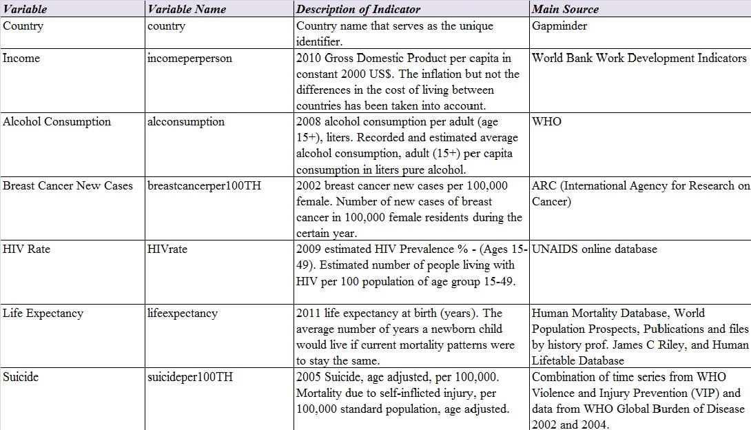
Please click here for my codebook.

Please click here for the entire SAS program. (Please click the following images for larger images)

1. Assign label names for variables

 

 

2. Set unknown values to missing values and create a secondary variable called HIVper100TH

 

 

3. Group values of the variables

 

 

4. Set range of values (completed in week 2) and interpreted responses (completed in week 3) for variables

 

 

5. Run frequency distributions tables that show groups of values

 

OUTPUT (FREQUENCY TABLES)

Please click here for all frequency tables.

 

Income per person by country was divided into 5 groups. 20% of countries had the lowest income per person of US$559 or less. The second group (21%-40% of countries) had income between US$560 and US$1,845. The third group (41%-60%) had income between US$ 1,846 and US$4,700. The fourth group (61%-80%) had income between US$4,701 and US$13,578. The 20% with highest income had income between US$13,579 and US$105,148. The range of income was larger for groups with higher income. There were no data for 23 countries, and those were marked as missing data.

 

 

 

 

 

 

 

 

The estimated average alcohol consumption per capita in liters were divided into 5 groups, 5 liters in each group. There were 43.32% of countries with alcohol consumption between 0 and 5 liters. There were 32.62% and 18.18% with alcohol consumption between 5.01 and 10 liters and between 10.01 and 15 liters respectively. There were only 5.88% with alcohol consumption between 15.01 and 25 liters. There were no data for 26 countries, and those were marked as missing data.

 

 

 

 

 

 

 

 

The numbers of breast cancer new cases in 100,000 females were divided into 5 groups. There were 28.9% of countries had 0 to 22 new cases. There were 39.31% and 17.92% had numbers of new cases between 22.1 and 44 and between 44.1 and 66 respectively. There were less countries with larger numbers of new cases; 9.83% and 4.05% had numbers of new cases between 66.1 and 88 and between 88.1 and 110 respectively. There were no data for 40 countries, and those were marked as missing data.

 

 

The estimated numbers of people living with HIV by country were divided into 5 groups. Secondary variable (HIV number per 100,000 people) was created from the primary variable (HIV rate/number in 100 people) because the numbers of breast cancer new case and suicide were presented with numbers “in 100,000 people”. 30% of countries had the lowest numbers of people living with HIV, between 0 and 100 people in 100,000 people. The second group (31%-40%) had the numbers of people living with HIV between 101 and 200. The third group (41%-60%) had numbers between 201 and 600. The fourth group (61%-80%) had numbers between 601 and 1,800. 20% with the highest numbers of people with HIV were between 1,801 and 25,900. The groups with larger numbers of people with HIV had larger range than the groups with smaller numbers of people with HIV. There were no data for 66 countries, and those were marked as missing data.

 

 

 

 

 

 

 

 

The average numbers of years a newborn child would live were divided into 5 groups, 10 years in each group. There were 4.71% of countries with life expectancy between 40.001 and 50 years of age. There were 15.18% and 19.9% with life expectancy between 50.001 and 60 years old and between 60.001 and 70 years old respectively. The highest percent of life expectancy (48.17%) were in the group between 70.001 and 80 years of age. There were 12.04% with life expectancy between 80.001 and 90 years of age. There were no data for 22 countries, and those were marked as missing data.

 

 

 

 

 

 

 

 

The numbers of suicide in 100,000 people were divided into 5 groups, 8 suicide cases in each group. There were 46.07% (highest percent) of countries with suicide numbers between 0 and 8. There were also 42.41% with suicide numbers between 8.001 and 16. The numbers of countries were decreased when the numbers of suicide increased. There were 11.52% with suicide numbers between 16.001 and 40. There were no data for 22 countries, and those were marked as missing data.

Data Management and Visualization – Running the SAS Program and Frequency Distributions

My SAS Program

Research Question: Is lower income associated with worse health from a global perspective?

Please click here for my codebook.

Please click here for the entire SAS program. (Please click the following images for larger images)

1. Call in a dataset, start the data step and assign label names for variables.

 

2. PROC steps: Set range of values for the quantitative variable called incomeperperson (2010 Gross Domestic Product Per Capita).

 

3. Set range of values for the quantitative variables called alcconsumption (Estimated Average Alcohol Consumption, Adult 15+  Per Capita Consumption in Liters Pure Alcohol) and breastcancerper100TH (Number of New Cases of Breast Cancer in 100,000 Females).

 

4. Set range of values for the quantitative variable called HIVrate (Estimated HIV Prevalence %, Age 15-49).

 

5. Set range of values for the quantitative variables called lifeexpectancy (Average Number of Years a Newborn Child Would Live) and suicideper100TH (Number of Suicide in 100,000 People).

 

6. Run frequency distributions.

 

Output (Frequency Tables)

Please click here for all frequency tables.

Description

There were a total of 213 countries (observations) in the Gapminder dataset. All 213 countries are included in this research. In terms of the income per person (2010 Gross Domestic Product per capita), there were 48.95% of the countries (93 countries) with the annual income between US$0 and US$2,500, 11.58% (22 countries) with income between US$2,500.01 and US$5,000, and 10.53% (20 countries) with income between US$5,000.01 and US$7,500.  In other words, there were 71.05% (135 countries) with income in the amount of US$7,500 or below. There were 28.95% (55 countries) with income between US$7,500.01 and US$107,500.  2010 Gross Domestic Product data from 23 countries were missing.

For the 2008 estimated average alcohol consumption for adults (15+ years old) per capita, there were 43.32% of the countries (81 countries) with the annual alcohol consumption between 0 to 5 liters, 32.62% (61 countries) with the consumption between 5.01 and 10 liters, and 18.18% (34 countries) with the consumption between 10.01 and 15 liters. There were 5.88% (11 countries) with the annual alcohol consumption over 15 liters. The alcohol consumption data from 26 countries were missing.

For the 2002 number of new cases of breast cancer in 100,000 females, there were 20.23% (35 countries) with the annual number of new cases between 10.1 and 20, 27.17% (47 countries) with the number between 20.1 and 30, and 16.18% (28 countries) with the number between 30.01 and 40. There were 33.52% (58 countries) with the number of new cases above 40. The breast cancer new case data from 40 countries were missing.

For the 2009 estimated percentage of people living with HIV, there were 90.48% (133 countries) with HIV prevalence between 0% and 5%. There were 9.52% (14 countries) with HIV prevalence above 5%.  The HIV prevalence data from 66 countries were missing.

For the 2011 life expectancy, there were 48.17% (92 countries) with the average number of years a newborn child would live between 70.001 and 80. There were 4.71% (9 countries) with the average years of age between 40.001 and 50, 15.18% (29 countries) between 50.001 and 60, and 19.90% (38 countries) between 60.001 and 70. There were 12.04% (23 countries) with the average years of age between 80.001 and 90. The life expectancy data from 22 countries were missing.

For the 2005 number of suicide in 100,000 people, there were 25.65% (49 countries) with the annual number of suicide between 0 and 5, 34.03% (65 countries) with the number between 5.001 and 10, and 26.70% (51 countries) with the number between 10.001 and 15.  There were 13.6% (26 countries) with the number above 15.  The number of suicide from 22 countries were missing.

Data Management and Visualization – Getting the Research Project Started

Data Set

I would like to work with the GapMinder data because I can find useful variables for my topics, income and health, from global perspective.

Research Question

Is lower income associated with worse health?

Hypothesis

There is a positive relationship between income and health. Lower income is associated with worse health. The variables including country, income per person, alcohol consumption, number of breast cancer new cases, HIV rate, life expectancy and number of suicide will be examined.

My Code Book

Variable as the Unique Identifier: Country

Variable for Income: Income Per Person

Variables for Health: Alcohol consumption, number of breast cancer new cases, HIV rate, life expectancy and number of suicide (suicide reflects poor mental health)

(Please click the image for larger variable table)

Literature Review

Search Terms Used: Income, health, poor

Summary of findings:  There is a positive relationship and bi-directional causality between income and health. Reduction in income inequality is associated with better population health.

Income variables used: Household income level, country income level, GDP, health expenditures, educational level, occupational level, employment status, Gini coefficients

Health variables used: Chronic conditions, self rated health, life expectancy, infant mortality, sex, age, race

Details of each reference:

(1)

Stronks, K., H. Van De Mheen, J. Van Den Bos, and J. Mackenbach. “The Interrelationship between Income, Health and Employment Status.” International Journal of Epidemiology 26.3 (1997): 592-600. Oxford Journals. Web. 10 Nov. 2015.

Link: http://ije.oxfordjournals.org/content/26/3/592.full.pdf

Research Question: Test the hypothesis that the relatively strong association between income and health, compared to that between education/occupation and health, can partly be interpreted in terms of an association between employment status and health.

Keywords: Socioeconomic inequalities in health, income, employment status

Variables: Proxies for income level including health insurance, housing tenure and car ownership, educational level, occupational level, employment status, 23 chronic conditions, self rated health

Findings: The relatively strong association between income and health can for a large part be interpreted in terms of an interrelationship between employment status, income and health. Income was still found to be related to perceived general health after controlling for employment status.

(2)

Erdil, E., and I. Yetkiner. “A Panel Data Approach for Income-Health Causality.” (2004): n. pag. 2004. Web. 12 Nov. 2015.

Link: http://fnu.zmaw.de/fileadmin/fnu-files/publication/working-papers/FNU47.pdf

Research Question: What kind of (Granger) causality relationship exists between health and income?

Keywords: Income, health, Granger Causality.

Variables: Real per capita GDP, real per capita health expenditures, country’s income level

Findings:  The Granger causality approach to panel data model with fixed coefficients was used to determine the relation between GDP and health expenditures per capita. The results showed the existence of bidirectional causality. However, this causality is not homogenous. The study showed a stronger evidence of bi-directional (Granger) causality running between health expenditure and income for a larger set of countries and by more refined econometric techniques. Moreover, one-way causality generally runs from income to health in low- and middle-income countries whereas the reverse holds for high-income countries.

(3)

Shmueli, A. “Population Health and Income Inequality: New Evidence from Israeli Time-series Analysis.” Oxford Journals. International Journal of Epidemiology, 23 Sept. 2003. Web. 12 Nov. 2015.

Link: http://ije.oxfordjournals.org/content/33/2/311.full.pdf

Research Question: What is the relationship between population health and inequality in income distribution?

Keywords: Population health, income inequality, Gini, income transfer, Israel, time series

Variables: Life expectancy at birth and at ages 5 and 65 for men and women, infant mortality, GDP per capita, educational level, national expenditure on health per capita, linear trend used to reflect medical-technological changes over time, Gini coefficients (Gini economic income, Gini pre-tax income and Gini disposable income)

Findings: None of the three income inequality measures (economic, pre-tax and disposable incomes) had an effect over time on population health. However, larger contemporaneous reductions in inequality, mainly through the transfers system, were associated with better population health, in particular with lower infant mortality.

(4)

Blakely, Tony A., Bruce P. Kennedy, Roberta Glass, and Ichiro Kawachi. “What Is the Lag Time between Income Inequality and Health Status?” Journal of Epidemiology & Community Health 318th ser. 54.4 (1999): 318-19. BMJ. Web. 10 Nov. 2015.

Link: http://jech.bmj.com/content/54/4/318.full

Research Question: What is the lag time between income inequality and health status?

Search Terms: Health, income

Variables:  Sex, age, race, equivalized household income, self rated health, Gini Coefficient

Findings: Although not conclusive, income inequality up to 15 years previously may be more strongly associated with self rated health than income inequality measured contemporaneously, for people aged 45 years and older at least.